EM Side-Channel Analysis of the EFR32MG12 Hardware AES Accelerator
Introduction
We used a near-field EM probe to recover an AES-128 key while the
Silicon Labs EFR32MG12's CRYPTO0 hardware accelerator performed decryption.
The setup uses a Rigol MHO98 oscilloscope, a NewAE probe and amplifier, and a
hobby CNC for positioning.
We couldn't quite get all 16 bytes reliably from correlation power analysis (CPA) alone. Even after tuning the capture and analysis, there was always one byte left to brute-force. In the run below, CPA recovered 15 bytes of the round-10 key. Searching the remaining byte and checking against a captured plaintext/ciphertext pair finished the job.
Most of the work went into getting usable traces. We started with software AES, spent about a month trying deep-learning approaches, then came back to CPA with better probe positioning and much more averaging. Raelize's Breaking HW-AES with Electromagnetic Analysis was the main reference. Their ESP32 work provided a useful starting point for both the position scan and the averaging strategy.
For these tests, we used a development board and firmware that lets us choose inputs, repeat operations, and trigger the scope with a GPIO. The package is intact. We used a known key to find a probe position and useful sample points, then tested recovery on a separate capture with a randomly selected key. That's a convenient setup to work with, and those conditions matter when considering whether the result applies to a real device.
Starting with software AES
The target firmware is a fork of ChipWhisperer's simpleserial AES example.
A Makefile switch, CRYPTO=SW|HW, selects TinyAES or the on-chip CRYPTO0
engine, so we could use the same command protocol for both. We started capturing
traces with a
ChipWhisperer Husky.
The target runs from its own 38.4 MHz crystal; the Husky's HS2 clock is not
connected.
CPA on TinyAES worked with a few thousand traces. For encryption, the model
HW(SBox(pt ⊕ guess)) recovers the master-key bytes. For decryption,
HW(InvSBox(ct ⊕ guess)) recovers the round-10 key, which can be inverted
through the AES key schedule to obtain the master key. All 16 bytes ranked
first in the software tests. The tools call that rank 0.
We moved the capture code out of the H-Field Probe Demo notebook into a
headless capture.py CLI, with Lascar handling CPA. We started with
ChipWhisperer's CWContainer glue and extracted it to avoid pulling IPython
and pandas into the script. Having both capture and analysis on the command
line made the later scans and long acquisitions much easier to automate.
Then we switched to CRYPTO=HW. With 15,000 traces, none of the models we tried
recovered a byte, and the best correlations were around 0.04. The setup that
worked for software AES wasn't giving us a useful hardware-AES signal.
Trying deep learning
During these experiments, we moved trace capture from the ChipWhisperer to the Rigol because we thought deep learning would need the higher sampling rate. The ChipWhisperer may have been enough, but we never went back to check.
We tried Google's SCAAML first, with a converter (cwp_to_scaaml.py) to turn
ChipWhisperer projects into training shards. Its scaaml_intro ResNet1D stayed
near the random-guess baseline: validation loss around 5.545, or ln(256).
Changing normalization and training for longer didn't get it past that.
Next we tried Ledger Donjon's SCADL approach, which uses CPA to locate points of interest, trains a small CNN on a window around each one, and combines candidate scores across attack traces.
That worked on software AES. The CNN ranked 12 of 16 bytes first, and a search of roughly 36 million candidates completed the remaining four in about two minutes. On hardware AES, though, validation loss stayed around 5.55 and none of the 16 bytes ranked first.
The software result gave us some confidence in the pipeline, but we weren't getting anywhere with the hardware traces. At that point, we put model training aside and worked on the measurements. Deep learning may still work on this target; the approaches we tried didn't recover the key from the traces we had.
Averaging and the test setup
Raelize averaged repeated operations with identical inputs to reduce noise. For independent noise, averaging K aligned measurements reduces its standard deviation by a factor of √K. At 1000 repetitions, that's about a 32-fold reduction under those assumptions. It also means collecting a lot of raw acquisitions: 200,000 averaged traces at 1000× represent 200 million AES operations.
Here's the setup we used:
- Target: an EFR32MG12 development board (SLWRB4161A + WSTK), running from
the 38.4 MHz HFXO. We bypassed the integrated DC-DC converter with
emuDcdcMode_Bypassbecause its switching dominated the EM measurement. PA2 supplies the trigger around the AES operation; input and RNG preparation happen outside that window. - Probe and amplifier: a NewAE planar H-field probe and low-noise amplifier, connected to scope channel 1.
- Positioning: a Genmitsu CNC 3018-PRO carrying the probe over the package.
- Capture: a Rigol MHO98. The Husky remains connected as the UART bridge to the target.
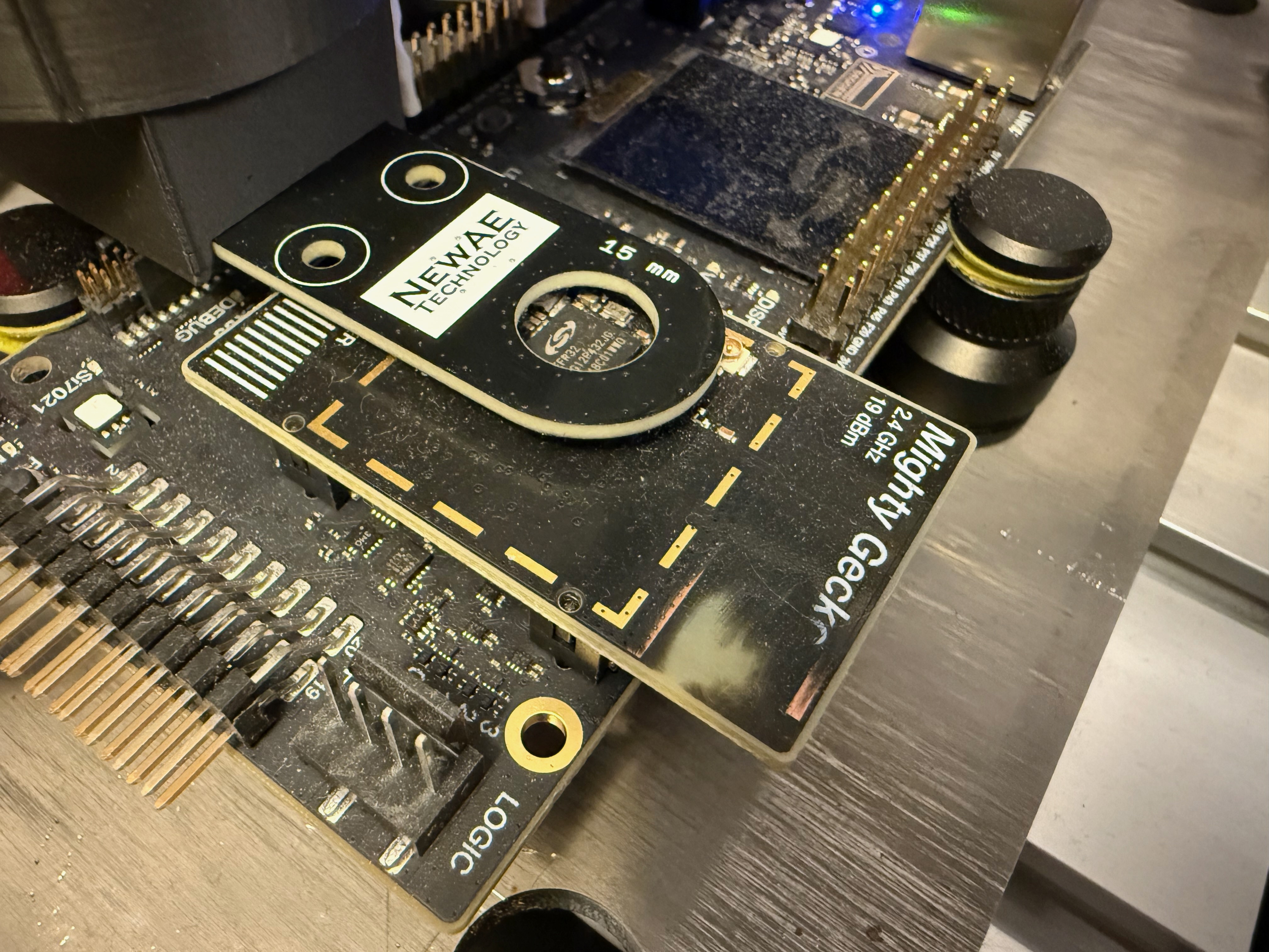
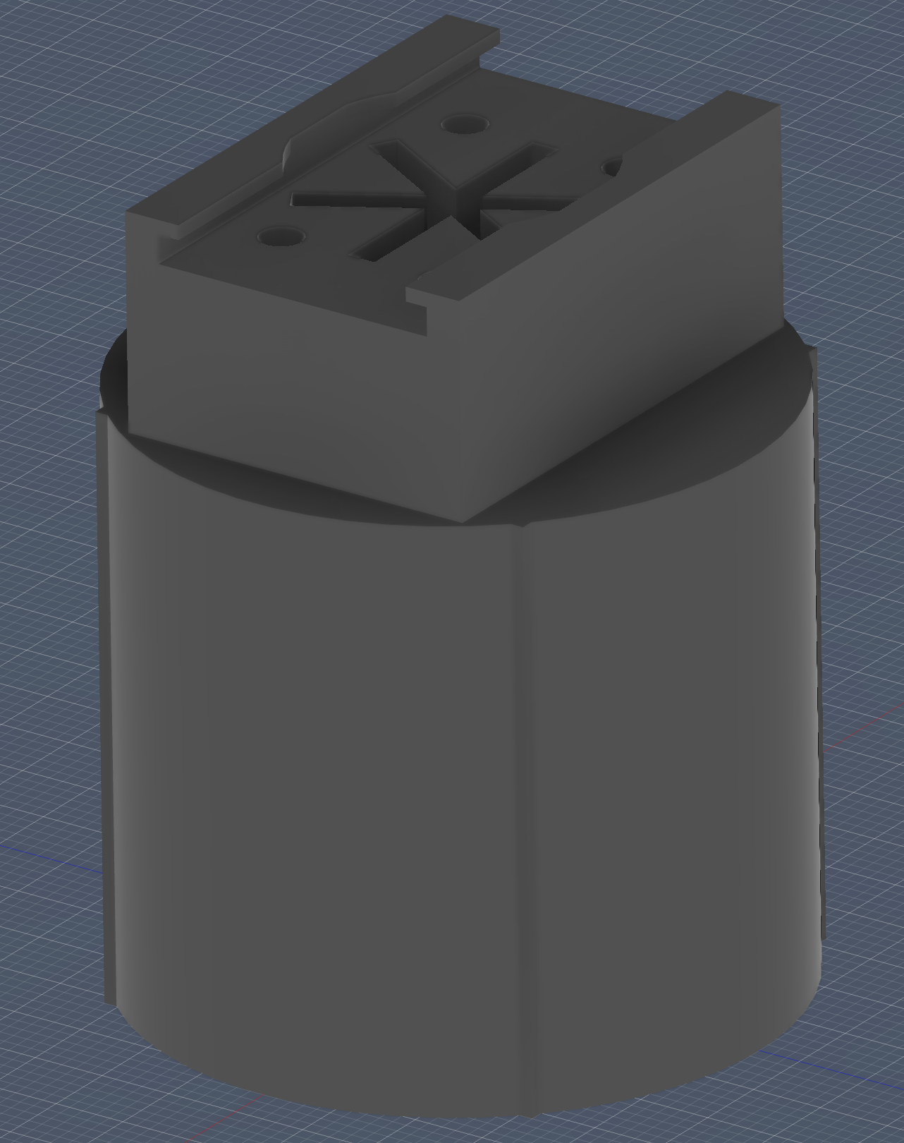
The probe over the target. The holder fits the CNC; the jig model shows its mounting arrangement.
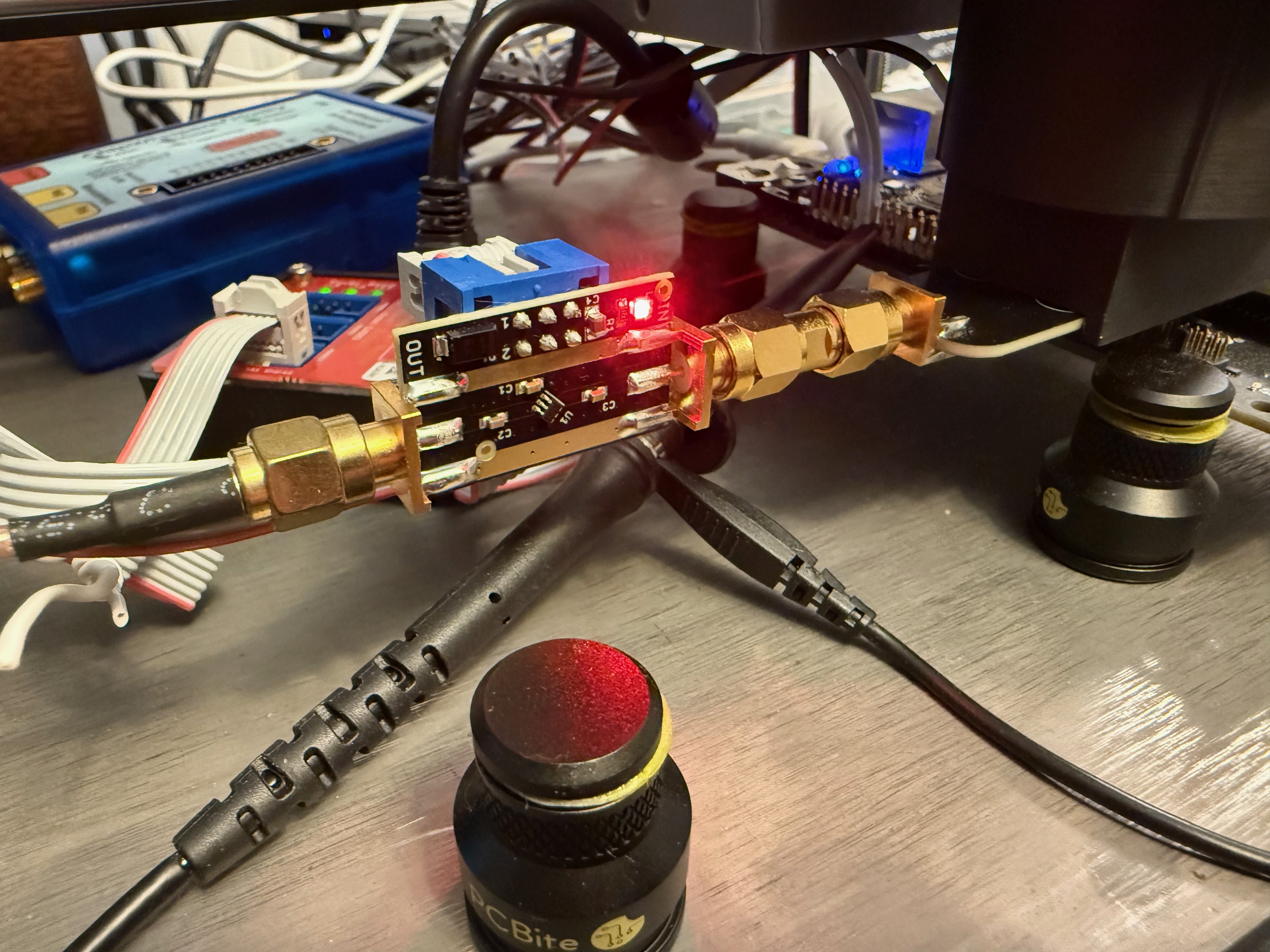
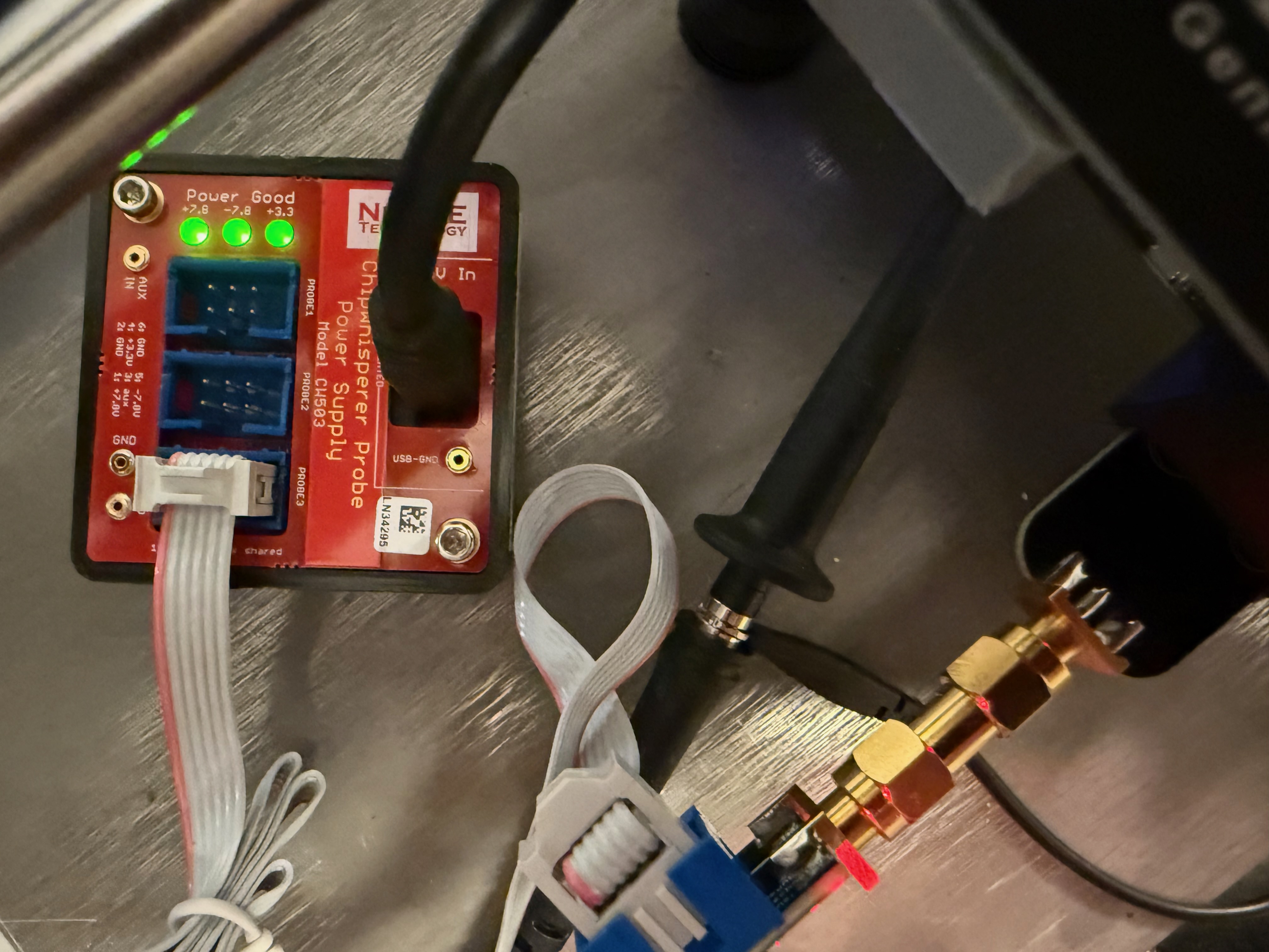
The amplifier in the measurement path. A separate NewAE probe power supply powers it.
Capturing and averaging on the Rigol
Arming and reading one trace at a time over SCPI gave us about 7 traces/s. That wasn't going to be practical at this averaging depth. The MHO's segmented acquisition mode, WaveRecord, can capture many frames in one session, but we couldn't find a stock interface for automating their bulk readback. The playback controls were in the UI, with CSV export available for saving a session.
After some time with the scope firmware in Ghidra, we used Frida to access
the frame buffers from the scope process. It took a few iterations to settle
on a native Frida CModule that reads the buffers and streams them to the host.
We eventually pulled this into a standalone package,
rigol-fastrec.
Internal DMA readback reached about 470 MB/s, while the built-in 100 MbE port delivered about 11.7 MB/s to the host. A Realtek RTL8153 USB Gigabit adapter raised that to about 27 MB/s. Network transfer was still the limiting step for raw readback.
So we moved the averaging onto the scope to send less data over that link. A NEON
accumulator in the Frida agent combines repeated frames before returning them
to the host, exposed as read(average=1000). The scope still has to acquire
every repetition, but only the averaged trace crosses the network.
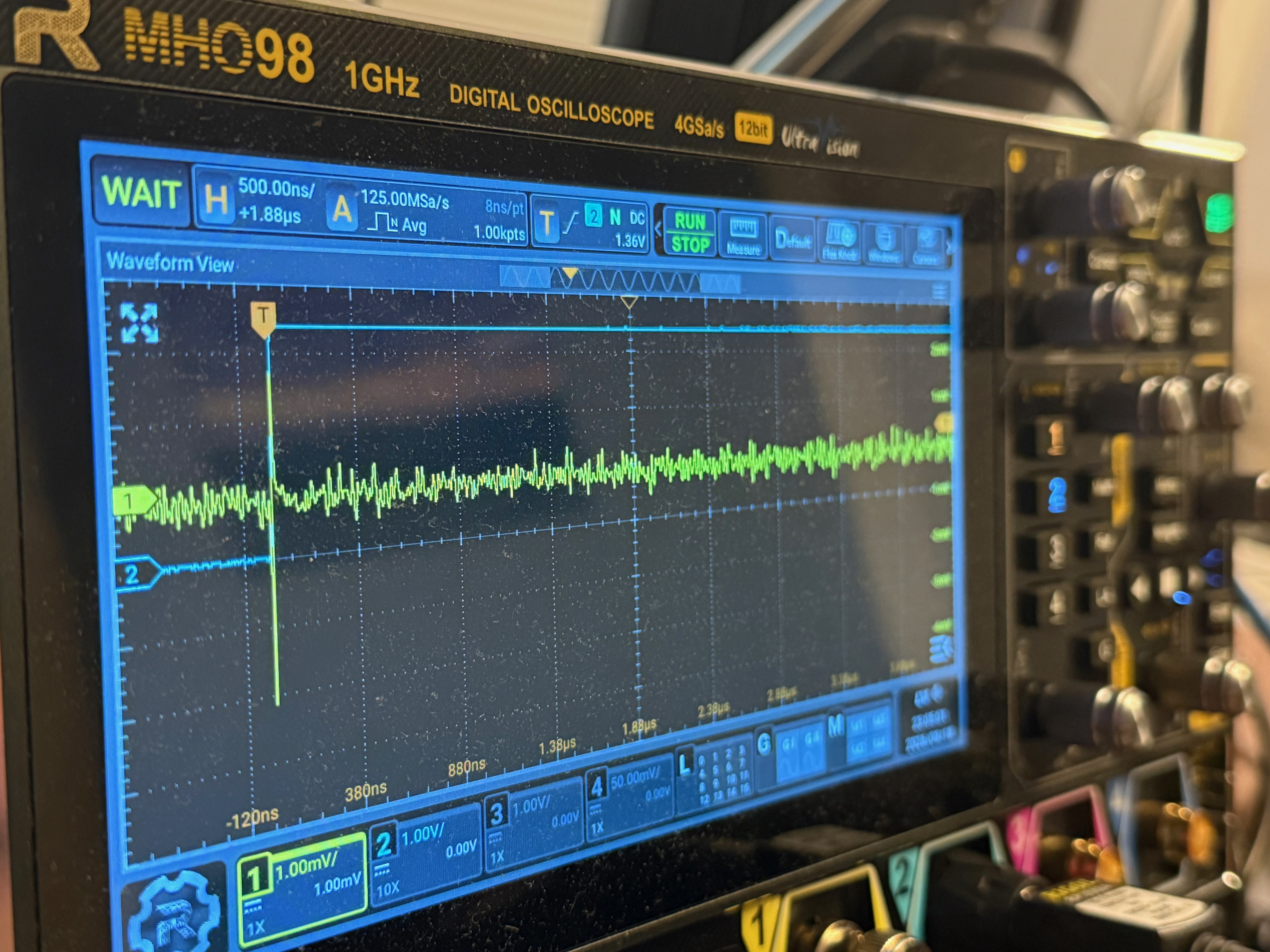
The scope during setup, displaying the EM signal and trigger. The screen settings in this photo are not the final capture settings below.
Along the way, we switched the capture and analysis tools to sedpack, the LZ4/FlatBuffer storage format used by SCAAML. That let us use the same analysis tools with traces from either the Husky or the Rigol.
Trigger timing and shorter records
Only about half the frames in our first bulk captures were usable. The triggered operation took about 7.8 µs, while each 10,000-sample record at 1 GSa/s covered 10 µs. The firmware was issuing triggers faster than the scope could finish and re-arm.
We added a delay-iters parameter to wait after each AES operation. For that
capture configuration, 60 iterations gave the scope enough time to keep up.
The delay sits outside the trigger window and needs to be tuned with the
record length.
With the timing sorted out, we captured 100,000 full-length traces and used known-key correlation to see which part of the record was useful:
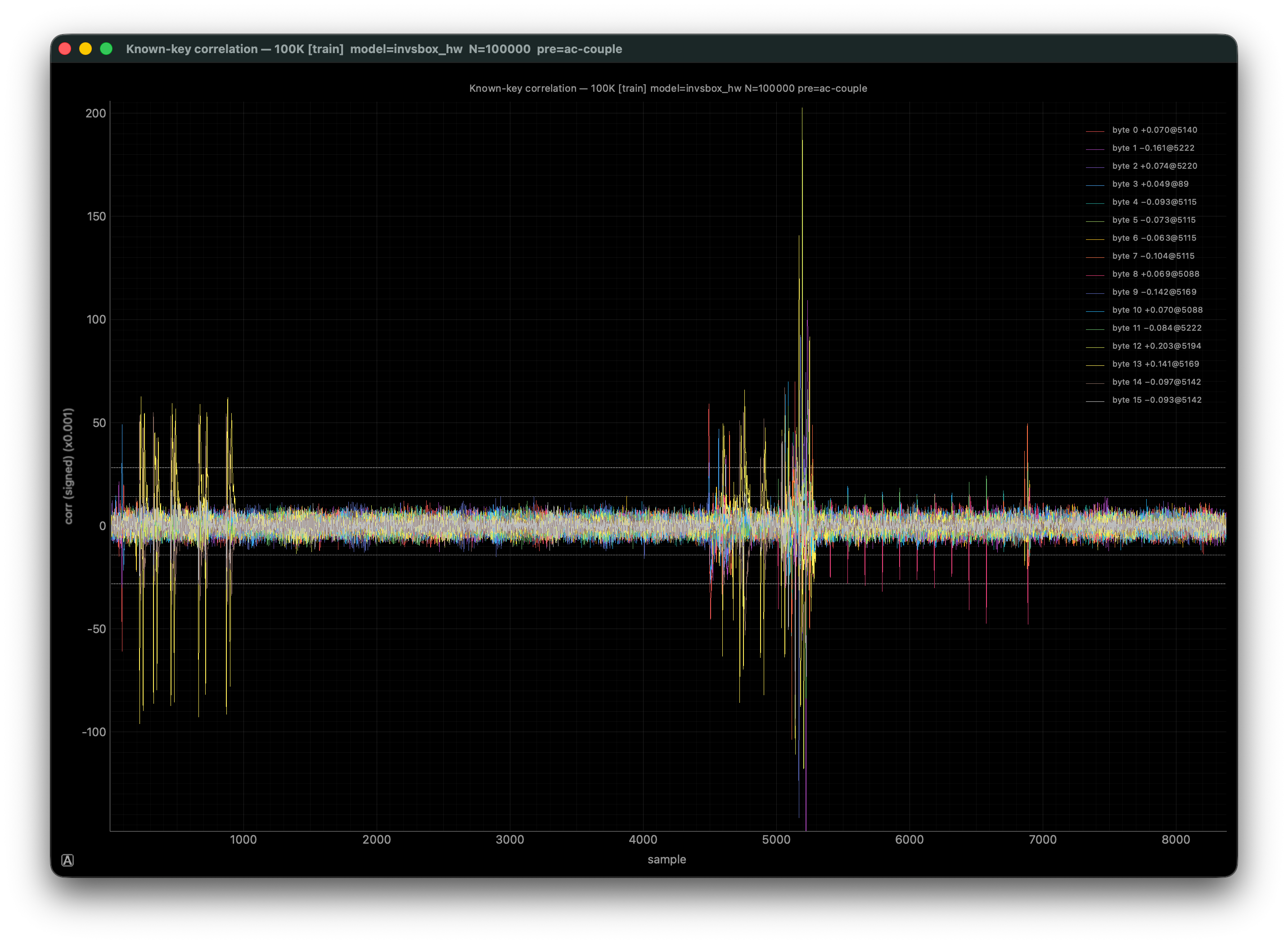
Full-window correlation from datasets/100K; the
saved log lists the per-byte peaks.
Selected lines from that output:
Loading train split from datasets/100K// ...
  100000 traces × 10000 samples each
  mode=decrypt  model=invsbox_hw
  preprocessing: ac-couple

  byte  1: peak corr=−0.1607 @ sample 5222
  byte  4: peak corr=−0.0930 @ sample 5115
  byte  9: peak corr=−0.1417 @ sample 5169
  byte 12: peak corr=+0.2027 @ sample 5194
Once we knew where to look, we could shorten the captures. For 200K_NARROW,
we reduced the record to 1000 samples, set a 5 µs trigger offset, and kept
samples 0:300 using the scope-side analysis_window. The agent averages and
crops before sending the result. That leaves 300 samples per stored trace
instead of 10,000, a roughly 33-fold reduction in data size on top of averaging.
Scanning the probe position
We used the CNC to scan an 8 mm square over the package, scoring each position
with known-key correlation using invsbox_hw on bytes 0, 4, 8, and 12. The
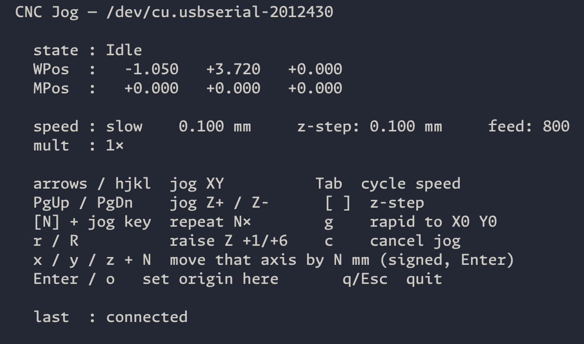
CNC jog interface handles manual positioning before a
scan.
The scan used a 30×30 grid, about 0.28 mm between points. At each of the 900 positions it collected 1500 averaged traces, with 1000 repetitions per trace and 1000-sample records at 1 GSa/s. That's 1.35 million stored traces from 1.35 billion raw acquisitions. At roughly 13,300 raw acquisitions/s, the scan took about 28 hours.
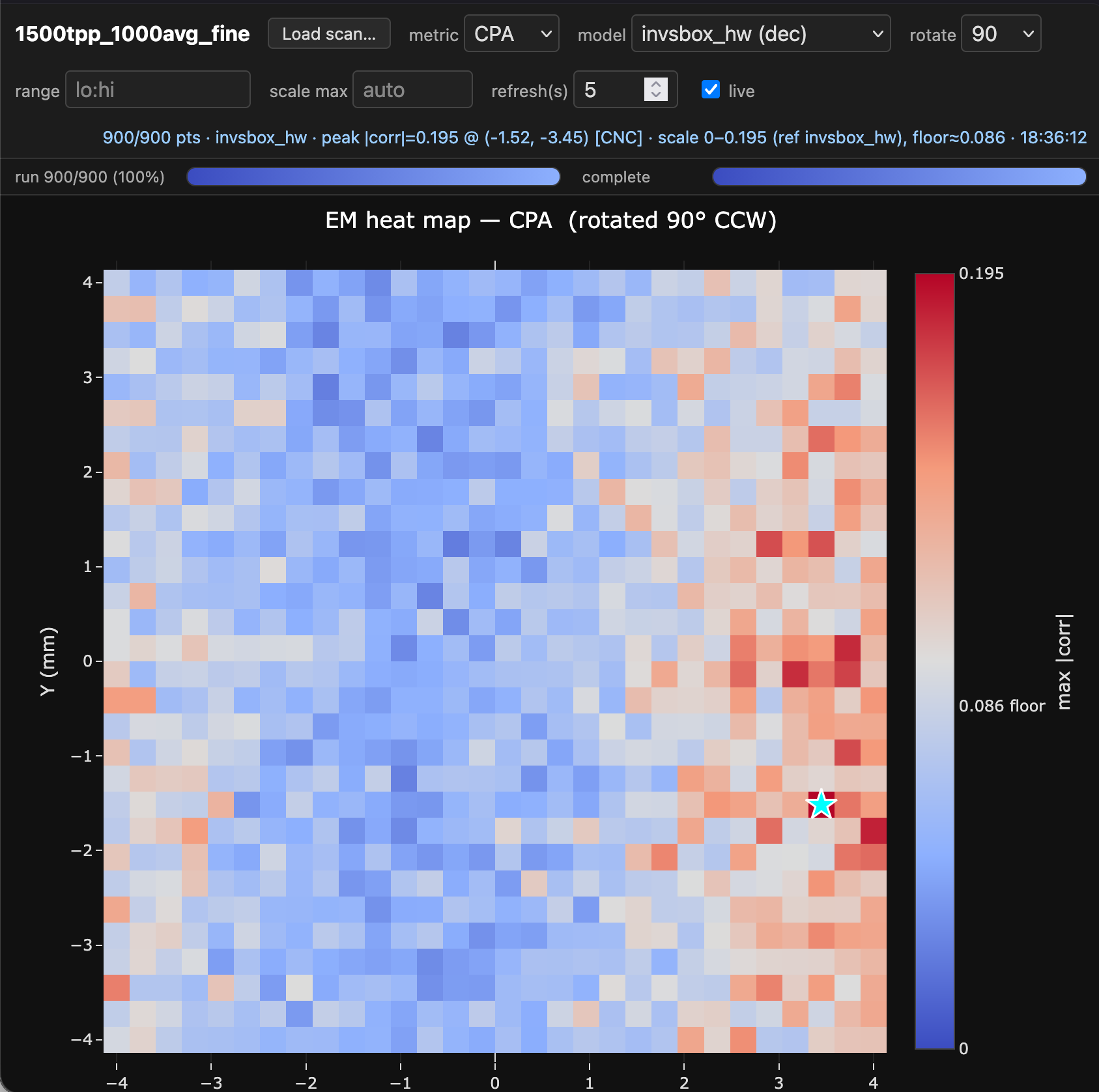
The scan dashboard, with the map rotated 90° counterclockwise. The selected peak is about 0.195 at CNC coordinates (−1.52, −3.45) mm, displayed as (+3.45, −1.52) mm on the rotated map.
The stronger correlation was concentrated toward one side of the package, so we parked the probe at the selected position for the next captures. We borrowed the grid and averaging settings from Raelize's experiment, which also took roughly a day to scan. The similar timing gives some context for the capture speed, though the chips and measurement equipment are different.
Inspecting the captures
We used the capture dashboard to keep an eye on progress and run CPA checks on saved datasets:
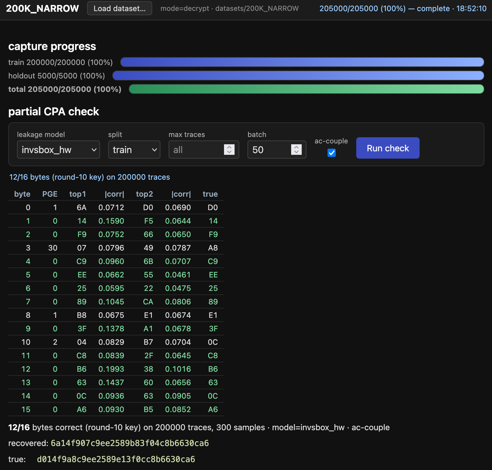
This is the earlier known-key 200K_NARROW capture, with 1000× averaging.
CPA over all 300 samples ranked 12 of 16 bytes first. It is separate from the
later 15/16-byte recovery run below.
Known-key correlation on this dataset shows where each byte leaks:
python cpa_plot.py --leakage-model invsbox_hw \
    --dataset-path datasets/200K_NARROW --ac-couple \
    --config config/efr32_hwaes_200k.json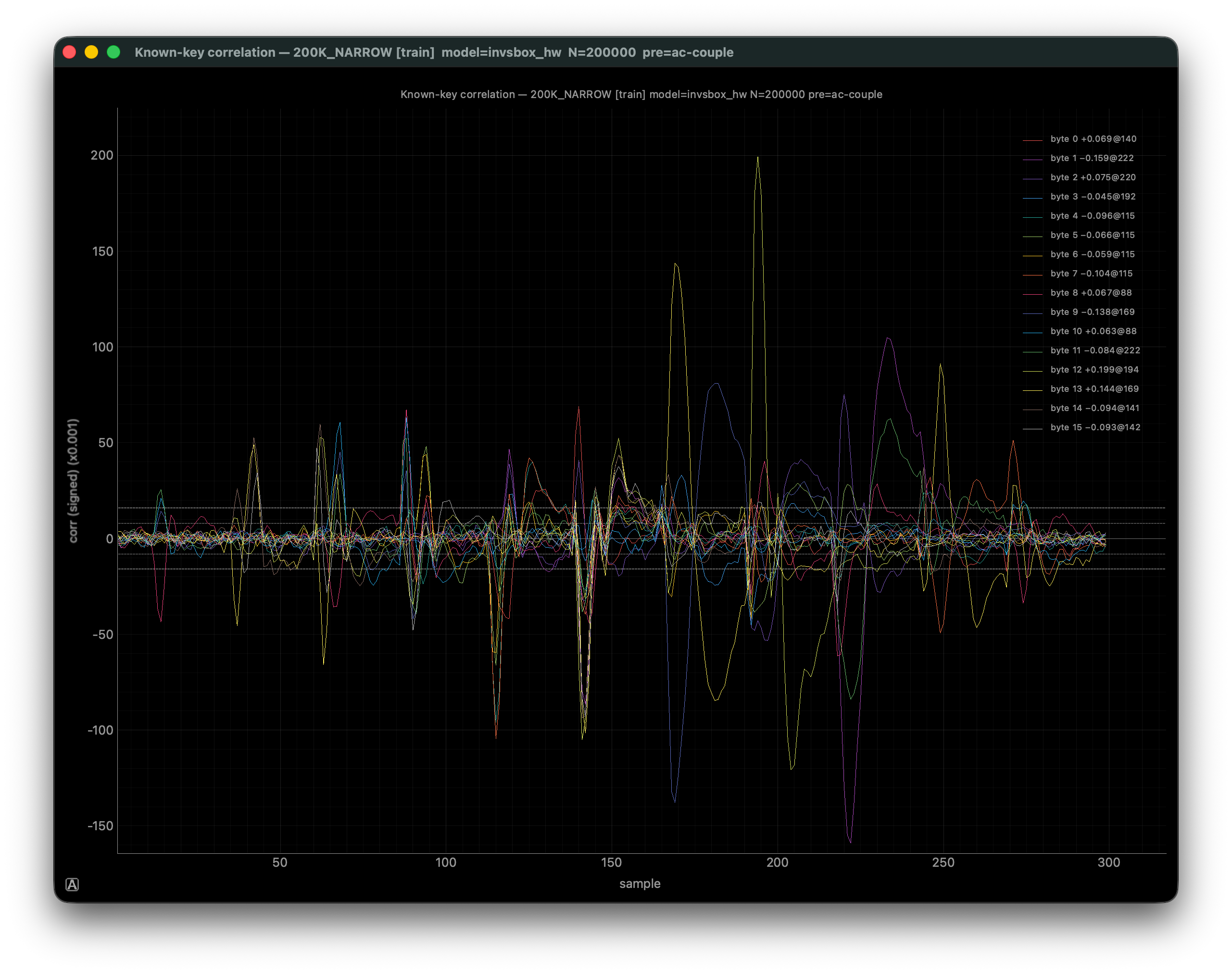
The narrower capture. Sample indices are relative to the 5 µs trigger offset; for example, sample 194 corresponds to sample 5194 in the full capture.
Selected lines from the narrow-window log:
  200000 traces × 300 samples each
  byte  1: peak corr=−0.1590 @ sample 222
  byte  4: peak corr=−0.0960 @ sample 115
  byte  9: peak corr=−0.1378 @ sample 169
  byte 10: peak corr=+0.0634 @ sample 88
  byte 12: peak corr=+0.1993 @ sample 194
Subtracting each trace's mean (--ac-couple) helped with baseline drift.
We also got better key rankings by restricting CPA to samples
115,169,192,194,220,222. In lascar_check.py, sample selection happens before
mean subtraction, so changing the window changes both the samples being scored
and the baseline used for centering.
One detail that took some care: a correlation peak for the known key doesn't guarantee that it beats all 255 wrong guesses. For example, near sample 88, byte 10's true value had a correlation of about 0.063, while a wrong guess reached about 0.083. We chose the six sample points using the known-key captures, then kept them fixed for the separate random-key capture.
Recovering 15 bytes and searching the last one
For the next run, we increased averaging to 2000 repetitions per trace and captured 200,000 traces under a randomly selected key. We kept the 300-sample records and the same six points for CPA. Here's the command from the recovery log:
python lascar_check.py --config config/efr32_hwaes_2kavg_unknown.json \
    --leakage-model invsbox_hw --ac-couple \
    --dataset-path datasets/200K_2KAVG_UNKNOWN/ \
    --analysis-window 115,169,192,194,220,222 \
    --blind-verify --brute-complete 3
Lascar took about seven seconds for the CPA pass. This is the result before brute-force completion:
byte  PGE   top1 |corr|   top2 |corr|   true
----  ---   ----  ----    ----  ----    ----
  0    23   80  0.0201    9F  0.0199    D9
  1     0   AD  0.0834    8E  0.0263    AD
  2     0   92  0.0238    9F  0.0203    92
  3     0   69  0.0843    E4  0.0262    69
  4     0   54  0.0378    36  0.0342    54
  5     0   B6  0.0902    01  0.0473    B6
  6     0   41  0.0493    85  0.0362    41
  7     0   9B  0.0750    5B  0.0589    9B
  8     0   00  0.0266    64  0.0132    00
  9     0   9A  0.1405    2D  0.0570    9A
 10     0   EF  0.0232    BD  0.0116    EF
 11     0   99  0.0286    61  0.0168    99
 12     0   BA  0.0329    1D  0.0279    BA
 13     0   CC  0.1156    7B  0.0470    CC
 14     0   3A  0.0306    74  0.0139    3A
 15     0   10  0.0462    9D  0.0176    10

15/16 bytes correct (round-10 key)
recovered: 80ad926954b6419b009aef99bacc3a10
true:      d9ad926954b6419b009aef99bacc3a10
Byte 0 was still wrong. Its true value, D9, was at zero-based rank 23, and
the top two guesses had nearly identical scores. Inverting the top guesses
through the key schedule produced a master key that failed the captured
plaintext/ciphertext checks.
The completion step orders bytes by the gap between their top two correlation
scores and searches the least confident byte first. Each candidate round-10
key is inverted to a master key and checked against a captured pair.
--brute-complete 3 permits escalation to three bytes if needed; this run
finished after searching only byte 0, a space of at most 256 candidates.
That was enough to finish the recovery:
  escalate k=1: brute-force weakest 1 byte(s) [0] (≤256 combos, PT/CT-validated)...
BLIND KEY RECOVERY COMPLETED ✓  1 byte(s) actually wrong: [0]
  round-10 key = d9ad926954b6419b009aef99bacc3a10
  master       = 5f82c2d9cfeb0fa321d7d982f8bd1045
The table's true and PGE columns use the stored key for diagnostics. Candidate
ranking, selection of bytes to search, and plaintext/ciphertext verification
don't use it. That's what we mean by blind recovery here. We had already used
a known key to work out the probe position and sample selection.
What we'd try next
We got the key, but never quite got the repeatable 16/16-byte CPA result we wanted. Even with 2000× averaging, there was still one byte to brute-force. It's a small search, but it shows how little margin we have on the weaker byte measurements.
We expect a better probing setup would help a lot: a more sensitive probe, a better LNA, and more repeatable control of probe height and orientation. We're already using a NewAE amplifier, so the next thing we'd try is upgrading the probe and amplifier together. We haven't tested that yet, so we can't say whether it would get us the last byte directly or how much less averaging we'd need.
For us, automating probe placement and averaging on the scope made the biggest practical difference. Once we had usable traces, CPA and a small candidate search were enough to recover the key.
Applying this to the original device
The development board was a stand-in for a commercial IoT device with encrypted firmware updates. We haven't recovered that device's firmware encryption key yet.
We don't have its source code. Based on its black-box behavior, our working assumption is that it stages an encrypted update in flash, checks a signature, and only then decrypts and installs it. If that's right, it limits the chosen-input access we relied on in these tests. Getting repeated captures with a useful trigger may also be much harder during an actual update.
A limited set of signed updates doesn't by itself rule out CPA: one image contains many AES blocks, and known inputs can be enough. We still need to work out whether we can identify those inputs, align the corresponding operations, and repeat the captures enough times for this setup.
The AES mode matters too. If the device uses CTR, the AES input is the counter block, and decryption uses the AES encryption operation. We'd need to work out that input and adapt the leakage model. We don't yet know how the device handles its IV/counter; that's a gap in our understanding of the device, not evidence that CTR prevents side-channel analysis.
So far, we've recovered a development-board key with CPA and a one-byte search. To apply that to the original device, we still need a workable way to capture traces and a better understanding of its update path.